This project focuses on creating a Recurrent Neural Network (RNN) to predict the upcoming faults in a wind turbine based on past failures and general data.
NOTE: the project work stream might be extrapolated, by applying minor modifications and/or fine-tuning procedures, to any new dataset (not limited to wind applications) containing failure information and reach applicable conclusions to real world.
The project is split in the following two parts, covering part 1 in this publication.
Part 1 is focused on next sections:
- INTRODUCTION
- DATA ACQUISITION
- CODE OVERVIEW
- RECURRENT NEURAL NETWORK CREATION
Part 2 is focused on next sections:
- SEQUENCE PREDICTION USING AUTOENCODER
- RNN MULTILABEL
- APPLICATION NETWORK CUSTOMIZATION
As reference, the code is entirely developed in Python using Keras/Tensorflow frameworks and is accessible from below link.
INTRODUCTION
Wind energy is an uptrend renewable source with significant market penetration, reaching almost 10% of worldwide electricity generation share in 2022, and +20% in the most developed European countries. That share is expected to increase, especially due to offshore wind farms with +10MW wind turbines expansion. As reference, one single spin of an offshore turbine might supply full day power for two homes of a developed country.
However, the outlook for wind energy can only be promising with high reliability performance and reduced cost of quality. A wind turbine is a very complex system with a large number of potential failures. Each failure is very expensive since wind turbine accessibility is limited, and even more limited when installed offshore, and might take days or weeks to be repaired. That is translated to high levels of lost energy and cost of quality.
In light of the above explanation, multiple work streams to improve wind turbine reliability performance has been launched. Thus, the present project focuses on the innovative approach to proactively anticipate the upcoming failures and reduce turbine cost of quality. If the upcoming failures are known, different strategies might be enabled to optimize downtime impact such as proactively modifying wind turbine operating conditions or combining several maintenance actions in the same turbine access. For that purpose, the present project introduces a complete development work stream to predict wind turbine upcoming failures, starting from a simpler generic neural network configuration and finishing with a more complex approach focused on optimizing the application under analysis.
DATA ACQUISITION
To generate the project dataset, data recorded for 3 years (from January 2021 to December 2023) for 21 wind turbines installed in Sweden was used as reference. However, due to confidentiality issues, failures are mapped with integer numbers to eliminate interpretability.
The project dataset has 812k rows and 637 unique failures. After deeper data exploration, there are a large number of failures only triggered in a specific turbine or failures with a very low total occurrence. To simplify and eliminate uncommon failures, the project dataset is generated after applying a scrubbing layer with the next functionalities:
- Unify blade specific failures instead of having and independent failure per each blade
- Focus only on failures with at least 30 occurrences in all wind turbines considered in the analysis
The final project dataset after the preprocessing layers described above has 523k rows and 33 unique failures. In turn, each row has 4 features: elapsed time from previous failure, failure identification number (ID) and both wind speed and wind turbine power when failure was triggered. Next picture depicts the failure occurrence distribution among the 523k rows. Failure IDs are highly unbalanced and needs to be managed to create a model with high generalization power, as it is discussed in next chapters.

Next table summarizes the number of failures detected corresponding to the turbine dataset rows per each wind turbine. Not all turbines are expected to trip the same exact number of times, but similar magnitude of rows is expected. Thus, except turbine number 2, which has a limited running time due to a major repair, all turbines has around 25k rows.

In the following, a global summary table with the percentage of each failure per turbine is depicted to have a better overview about failure distribution. Each row represents a turbine and each column represents a failure ID, so the sum for each row is 100%. The results show a significant unbalanced failure distribution trend in all turbines, being failures ID 10, 11, 12 and 13 the most common with >50% total failure share. However, the trend is constant in all turbines and validates the data homogeneity among turbines.

CODE OVERVIEW
The code is entirely developed in Python using Keras/Tensorflow frameworks and consists of the next Python files.
- RNN.py: main file to define simulation features and parametrization. Moreover, it manages the simulation execution by calling functions, metrics and loss functions from the rest of files.
- custom_metrics.py: available open metrics and loss functions did not fully satisfy the project requirements and so, this file captures in-house metrics and loss functions using Keras backend and Tensorflow functions.
- display.py: it is a collection of visualization functions (as plots, graphs, tables or matrix) to generate the required visual output to understand simulation performance.
- utils.py: it is a collection of specific purpose functions (as preprocessing, data scrubbing or neural network creation) to help optimizing code refactoring and understanding.
As observed in previous chapter, dataset is highly unbalanced. If no action, loss function would intrinsically provide higher weights to most common failures, achieving a great learning power for these failures, but ignoring the low occurrence failure patterns, which would lead to a mediocre macro average performance. To mitigate that undesired effect, the next in-house weighted_crossentropy_loss loss function was developed.
- The loss requires an input weight 1D-array indicating the crossentropy loss multiplier to each output class. Note the default unweighted scenario would correspond to an input weight array [1, 1, ..., 1].
- The function accepts both binary and categorical applications. When working on binary applications and with the purpose to maximize the effect of positive outcome in low occurrence failures and negative outcome in high occurrence failures, the weights are directly applied for positive targets and inversely applied for negative targets. Note binary loss expects sigmoid as output activation layer and categorical loss expects softmax.

Weights array calculation is managed in the next weight_calculation function, accessible in utils.py. With the purpose to reinforce the learning power of detected critical failures, the function allows adding extra multiplier effect in certain failures using crit_ids and multiplier input parameters. During the project development, the next four weighting approaches are considered.
- Unweighted: defines a [1, 1, ... , 1] weight array.
- Natural Logarithm-weighted: defines unit weight to the most common failure, and increasing weights according to the natural logarithm factor for each failure vs the most common one. This is the default approach.
- Mean-weighted: defines unit weight to the mean occurrence failure, and increasing or decreasing weights according to the factor for each failure vs the mean occurrence one.
- Mix-weighted: defines weight array based on averaging weights from natural logarithm and mean approaches.

Simulation parametrization is captured in the variable sims, which accepts the below inputs . Note sims might be in fact a nested list and run multiple different simulations in the same code execution.
- Application: to select application to simulate (RNN single-label, Autoencoder or RNN multilabel).
- Output_seq: length of the output predicted sequence.
- Units1/Units2: number of neurons for first and second RNN layer (0 to disable a layer).
- Dropout: value to use for both dropout and recurrent dropout.
- Max_samples: maximum allowable samples per a single failure (-1 if no undersampling).
- Learning_rate: learning rate to apply during training.
- Batch: batch size. Current literature aims to lower batch size to maximize generalization learning power. However, to have at least a representative number of samples for all classes in each training step, batch size for current application cannot be low given the high data unbalanced degree. Therefore, batch size is defined to 512 for the project development.
- Embedding_size: positions of the failure embedding vector (0 to use one hot vectors instead of embedding)
- Lookback: number of past samples to focus when predicting new ones.
- Weighted_loss: weight approach to use for crossentropy loss calculation.
- Critical_ids: list of critical IDs to reinforce learning power by adding an extra multiplier to the original weight.
- Critical_multiplier: multiplier to use in the critical failure IDs.
- Threshold: minimum probability to consider true predictions (valid for chapter Application Network Customization).
RECURRENT NEURAL NETWORK CREATION
This chapter focuses on creating a multi-class single-label recurrent neural network to predict the immediate upcoming next failure among the 33 different failures in the dataset. To capture both past failure data and data as wind speed, power and elapsed time among failures, a multi-input neural network is used. Each input follows the next work stream.
- Past IDs data: depending on simulation settings, it is either one hot encoded or applied to an embedding layer.
- Input data: wind speed and wind turbine power are one hot encoded into three features (high-speed, medium-speed and low-speed), and two features (turbine on and turbine off), respectively. Elapsed time among failures is standardized. Therefore, input data is captured with a total of 5 features.
Then, both data are concatenated prior to apply RNN layer(s) with ReLU as activation function. GRU units are selected for the project development due to attractive trade-off between performance and computational cost. Output is a Dense layer with 33 neurons corresponding to the number of different failures and softmax as activation function due to the single-label approach. As an example, next picture depicts a multi-input RNN diagram with 100-position embedding layer for the past IDs data and two linked GRU layers of 128 neurons each.

For training and tuning purposes, dataset is split into training, validation and testing sets, with 80-10-10% splits, using a stratified approach by calling the function stratified_train_val_test_split from utils.py.
RNN input and target data are yielded through a generator in the form of [input data, past IDs data], target data implemented in the function generator from utils.py. This function yields the corresponding batch size packages for each simulation step. However, the detailed work to pack data per simulation settings is managed in the function data_preparation from utils.py according to parameters as lookback, lookforward and output sequence length. As reference, below picture emulates a particular example for a data generator packaging process with batch size = 3, lookback = 6, lookforward = 6, 5 input features and an input sequence length with 17 timesteps.

- First sample to input in the neural network focuses on time step 5 since lookback is 6. Therefore, input data for first sample includes data for all input features for timesteps 0-1-2-3-4-5. Instead, target data for first sample includes the information to predict referred to timestep 11 since lookforward is 6 and current timestep is 5.
- Similarly, second sample is referred to timestep 6, having as input data the data for all input features for timesteps 1-2-3-4-5-6, and as target data the information to predict referred to timestep 12.
- Finally, third sample is referred to timestep 7, having as input data the data for all input features for timesteps 2-3-4-5-6-7, and as target data the information to predict referred to timestep 13.
- The package of the previous three samples is yielded by the generator to input the neural network for the first simulation step. Then, there is a second simulation step with a new set of 3 samples yielded by the generator corresponding to timesteps 8-9-10 with information to predict referred to timesteps 14-15-16.
- The two simulation steps with 3 batch samples each corresponds to a simulation run along the input sequence, known as epoch. To ensure a proper training, 50 epochs are considered in the project development, but linked to an early stopping callback to avoid overtraining or more commonly known as overfitting.
Loss function to train and tune the neural network is weighted_crossentropy_loss with natural logarithm weighting approach introduced in previous chapter. As for network performance, the next in-house metrics are created in the custom_metrics.py file.
- TPR_TOTAL: True positive ratio calculated as number of correct predictions vs number of total samples.
- PRECISION_TOTAL: Precision calculated as number of correct predictions vs number of total predictions. Note for the current application it matches to TPR_TOTAL since there is a prediction for each sample.
- TPR_MACRO: True positive ratio calculated as the average for all true positive ratios of each output class.
- PRECISION_MACRO: Precision calculated as the average for all precision ratios of each output class.
- F1_MACRO: F1 score calculated as the average for all F1 scores of each output class.
Note total metrics are only for reference since they do not accurately capture network generalization power due to the high data unbalanced degree. Therefore, macro metrics are the drivers for the tuning process decisions. TPR focuses on the quantity of correct predictions and precision on the predictions quality, so F1 score is considered the preferred metric by weighting both quantity and quality.
A total of 25 simulations with different settings has been performed. Below table captures a high-level summary of all simulations. The simulation number 23 reaches the highest F1 score for both validation and testing sets with a value above 0.59, close to training F1 score, and confirming correct generalization learning power and fitting. This simulation corresponds to a neural network with one GRU layer of 128 neurons, dropout 0.2, learning rate 0.001, lookback 10, no undersampling, 100-positions IDs embedding, natural logarithm weighting for loss calculation and a 2x factor in the weights for ID 6 and 8. The following sections details step-by-step the RNN tuning process to reach the definitive configuration.


NETWORK ARCHITECTURE
Network architecture definition is one of the first decisions when facing a deep learning task. If a network does not show overfitting trend without regularization, the network capability might be insufficient for the present application. The design procedure is to start with a small network and keep increasing capability until showing a clear overfitting trend. Simulations 1 to 4 capture this assessment, in which networks with single GRU layer of 32, 64 and 128 neurons and with dual GRU layers of 64 units each are tested.
Next picture shows the loss function results for a network with single GRU layer of 32 neurons vs 128 neurons. The 32 neurons network reaches epoch 50 without hitting early stopping since the validation loss keeps decreasing in parallel to training loss, so there is no overfitting. Instead, the 128 neurons network stops improving validation loss around epoch 20 until hitting early stopping callback in epoch 27, showing a clear overfitting trend. Therefore, a network with single GRU layer of 128 neurons is considered for further tuning. Note network with dual GRU layers of 64 neurons each might be also a valid option in terms of capability, but it reached slightly worse metrics results.

DROPOUT
Next step after defining network architecture is to apply regularization to mitigate overfitting and maximize network performance. The overfitting is mitigated in the present project by setting an early stopping callback linked to validation loss function and by using both dropout and recurrent dropout. To define the proper level of dropout, a sweep between 0.1 and 0.3 is performed captured in simulations 5 to 7.
Dropout 0.1 still shows an overfitting trend because validation loss stuck but training loss keeps decreasing. Instead, by increasing dropout to 0.2 both validation and training losses follows a similar trend. Therefore, dropout 0.2, leading to macro average F1 score = 0.55 for both validation and testing set, is considered for further tuning.

LEARNING RATE
Once the network architecture is defined and overfitting mitigated, some RNN hyperparameters can be tuned. Learning rate must be properly set to reach optimal performance, otherwise neural network might become unstable with high learning rates or not complete the training process with low learning rates. Therefore, simulations 8 and 9 add a positive and negative offset in learning rate from baseline scenario.
On a hand, low learning rate defined to 0.0001 leads to a clear under-performance vs baseline, only reaching macro average F1 score = 0.5 for both validation and testing sets. On the other hand, high learning rate defined to 0.005 did not lead to a clear under-performance, but it did not provide further benefit in validation and testing performance. Thus, learning rate is kept to baseline value of 0.001 for further tuning.
EMBEDDING
All previous simulations focused on applying one hot encoding to failure ID data. However, applying an embedding layer might lead to more optimal results. Simulation 10 changes one hot encoding preprocessing for a 100-positions Embedding layer to preprocess failure ID data. Results are better reaching a validation and testing macro average F1 score = 0.56, so further simulations will be based on failure ID embedding preprocessing.
LOOKBACK
All previous simulations run under the assumption to focus on the 5 past failure IDs to predict the upcoming one. Instead, simulation 11 extends the lookback range to the 10 past failure IDs to check if that generates further learning power. Results of setting lookback to 10 depict a clear positive effect reaching a validation and testing macro average F1 score close to 0.59, but at the same time the computational cost has been negatively affected. In case of having enough resources, higher lookback might be tested. However, that work stream is not captured in the present project due to the limited computational resources and the academical background, and a lookback of 10 will be considered for further tuning. Note that trade-off between performance and computational cost is one of the most common decisions in any machine learning or deep learning application.
Below table creates a checkpoint with the current best neural network design.

Further detail of the current best model performance is provided below with the testing set confusion matrix and classification report, created by calling the functions plot_confusion_matrix and plot_classification_report from display.py. Confusion matrix allows easily identifying the diagonal containing true predictions, but given the high data unbalanced degree does not provide a perfect visual performance interpretability. Instead, classification report provides clearer performance results. As expected, the most common failure IDs (10 to 13) have high TPR and precision ratios. However, performance of the rest of IDs is acceptable with most of them exceeding the 50% F1 score, except ID 6 and 8 which only reach around 20% F1 score and a TPR ratio barely above 10%. Note these low performer IDs will be managed individually later.


LOSS FUNCTION WEIGHTS
Previous simulations run use natural logarithm as loss function weighting approach. However, simulations 12 to 14 compares different weighting approaches as mean, mix and unweighted. Results for each weighting approach is captured next.
- Mean weighting approach provides strongly higher weights in the most uncommon IDs, which leads to increase the macro TPR ratio in exchange to highly reduce macro precision, reaching a mediocre macro F1 score = 0.51. Therefore, a very strong trend to force neural network focusing on low occurrence IDs enables more low occurrence classes to be correctly predicted by creating a prediction bias for these classes, leading to an inferior network performance.
- Natural logarithm weighting approach provides softly higher weights in the most uncommon IDs. That subtle weight modification leads to the best macro performance with a macro average F1 score =0.59 and so, it will be used for further tuning. With this approach neural network pays more attention to low occurrence IDs to learn some new patterns, but without creating a prediction bias with negative consequences in performance.
- Mix weighting approach provides weights not as increased as mean weighting, but also not as reduced as natural logarithm approach. It provides a middle point performance among the two previous approaches, increasing macro TPR ratio without a sharp penalization in macro precision and F1 score.
- Unweighted approach applies a unit weight to all failure IDs, leading to an acceptable performance and learning very well the most common IDs patterns due to the high data unbalanced degree.

As reference, classification report for mean weighting is depicted below to highlight the low occurrence IDs bias.

UNDERSAMPLING
Other potential approach to mitigate a high data unbalanced degree is to apply undersampling. However, that is not normally a preferred approach because it works basically reducing the training set by eliminating high occurrence IDs samples. Thus, simulations 15 to 22 focus on exploring the performance to apply undersampling in the training set to limit maximum samples per ID to 25k, 35k, 50k and 70k with both natural logarithm and unweighted approaches for loss function weighting.
Results are between macro average F1 score 0.56 and 0.58, so there is no improvement regarding the current best model, which was 0.59, and so undersampling approach is not implemented in the definitive network version. However, if an unweighted loss function was selected, undersampling to limit training set to a maximum of 35k samples per ID would lead to better results than the non-undersampled baseline scenario.
CRITICAL IDs
Last step focuses on improving performance of the detected low performer IDs 6 and 8, whose TPR ratio was only 12 and 18%. To do that, the weights of these two IDs are multiplied by two by defining the input parameter critical_ids = [6, 8] and critical_multiplier = 2. Note IDs 6 and 8 are selected in this particular case to pursue the best macro performance model for academical purposes, but weights should be tuned and customized according to real application needs and benefits.
Simulations 23 to 25 focus on increasing the weights of these IDs and adjusting dropout, but the best results, depicted below, are keeping dropout to 0.2. TPR ratio for IDs 6 and 8 has increased to 36% and 33%, but it comes in exchange to reduce precision. Higher increase in these IDs weights will have a negative bias effect by reducing further precision in exchange of progressively lower TPR increases. However, multiplier of 2 slightly improves macro average F1 score and that is included in definitive model.

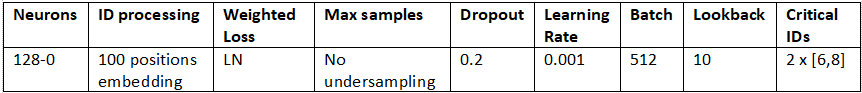
As summary, current chapter details a step-by-step procedure to develop, configure and tune a RNN for unbalanced applications, including assessing different strategies and hyperparameters sweeps to finally reach the most optimal solution. The definitive neural network is configured as follows reaching a macro average F1 score >0.59 in both validation and testing sets. Macro TPR and precision is around 0.59 and 0.6, and total accuracy 0.79.
NEXT STEPS
This publication has created a RNN to predict the next upcoming failure in a wind turbine using data for 21 wind turbines installed in Sweden for a recording time of 3 years. The final dataset presented a high unbalanced degree and mitigation actions were performed to force neural network paying more attention to patterns for low occurrence failures. For example, an in-house weighted crossentropy loss function was created to assign higher weights to low occurrence failures. Also, a critical weight multiplier was considered to boost performance for failures with low values in assessment metrics.
A RNN single-label neural network was developed, configured and tuned, including assessing different strategies and hyperparameters sweeps to finally reach the most optimal solution. The definitive neural network is configured to maximize macro average F1 score and ensure a proper learning power for all failures. In-house metrics were developed to assess model performance.
However, predicting just the immediate next failure might be a non-optimal scenario for a wind turbine application. Therefore, project part 2 focuses on modifying the RNN single-label architecture to provide a more general overview of the upcoming failures instead of just focusing in the next immediate failure.
I appreciate your attention and I hope you find this work interesting.
Luis Caballero
